One of the most common questions investors ask is, “what percentage of your trades are winners?” It sounds perfectly reasonable. And honestly, it’s the same question I would have asked a few years ago. We’re wired to think in terms of accuracy. In school, 90% means you aced it, 50% means you barely scraped through. So naturally, when people hear that a strategy wins only 40% of the time, their first instinct is to run.
If you’ve ever scrolled through fintwit or a Telegram group and seen someone flexing a 75% win rate, you’ve probably felt that pull. That must be a great strategy. But what if I told you that a trader winning only 4 out of every 10 trades could be making more money than the guy winning 6 out of 10?
That instinct confuses hit rate with expected value. And the distinction matters. Let me show you why.
A simple experiment
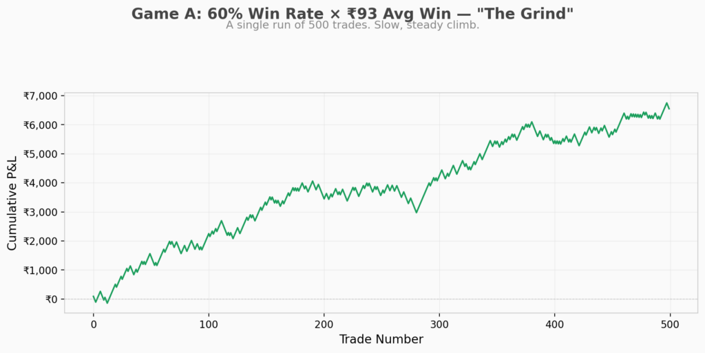
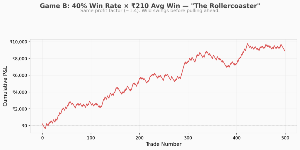
Imagine two coin toss games. Game A has a 60% win probability, paying ₹93 on a win and costing ₹100 on a loss. Game B has a 40% win probability, paying ₹210 per win with the same ₹100 loss.
Both have a profit factor of roughly 1.4. But the structure underneath is completely different.
Game A has a payoff ratio of 0.93, meaning each win is actually smaller than each loss. It makes money through frequency. Small margin, high volume. Game B has a payoff ratio of 2.10, making less frequent but significantly larger wins. It makes money through magnitude. Fewer trades, but each one counts.
The expected value per trade tells the real story.
Game A: (0.6 × ₹93) − (0.4 × ₹100) = ₹15.80 per trade
Game B: (0.4 × ₹210) − (0.6 × ₹100) = ₹24.00 per trade
Both positive. Both profitable. But Game B, despite its lower win rate, has the higher expected value per trade. If you’d dismissed it at “only 40% winners,” you’d have walked away from the better game.Put differently, expected value answers a simple question. If I played this game a thousand times, how much would I make on average per play? It weighs both the wins and the losses by how often each happens. A strategy with a 40% win rate and a ₹210 payoff is not losing money 60% of the time. It is investing in losses the way a venture fund invests in startups. Most individual bets don’t pay off, but the ones that do more than cover the rest. The logic is identical to staying in a SIP through a market dip because you trust that the probability of the markets giving you a positive return is higher in the long run, thereby, making your expected value higher. Only difference here is that it applies trade by trade instead of month by month.
What it feels like to play each game
Numbers on a spreadsheet are one thing. Watching your P&L in real time is another.
If you’ve ever held a position overnight, you know the feeling. You check your phone at 9:16 AM, see red, and your stomach drops. Now imagine that happening 10, 12, even 15 trades in a row. That’s the reality of Game B. Not because the strategy is broken, but because a 40% win rate means you will go through stretches where it feels like nothing works.
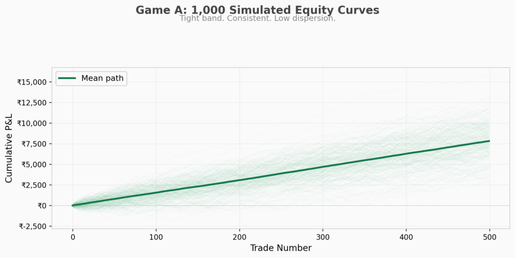
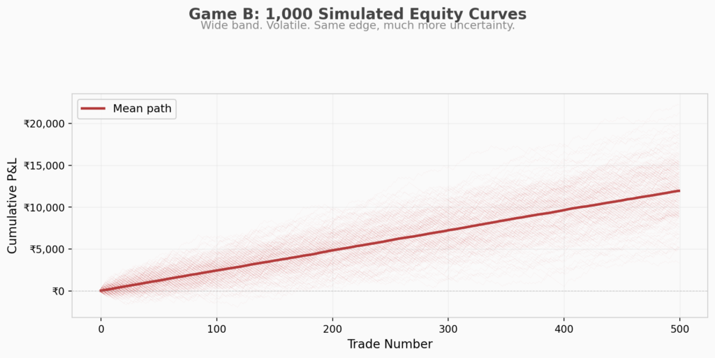
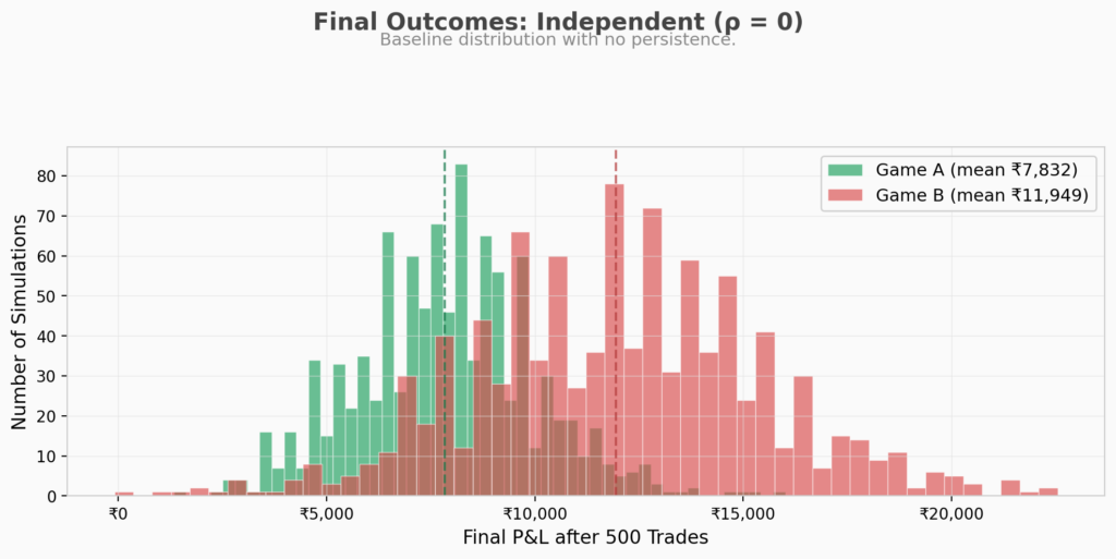
Game A, on the other hand, feels like a SIP that’s always slightly in the green. Small wins stack up. Losing streaks top out at 6 or 7 trades. It’s boring. It’s comfortable. And for most retail traders, that emotional smoothness is worth more than they realise.We ran a Monte Carlo simulation. 1,000 iterations of 500 trades each. Both games were profitable in 100% of simulations. But the experience of playing them is night and day.
Same edge. Same profit factor. One feels like rotating the strikes and taking singles. The other feels like swinging for sixes every ball.
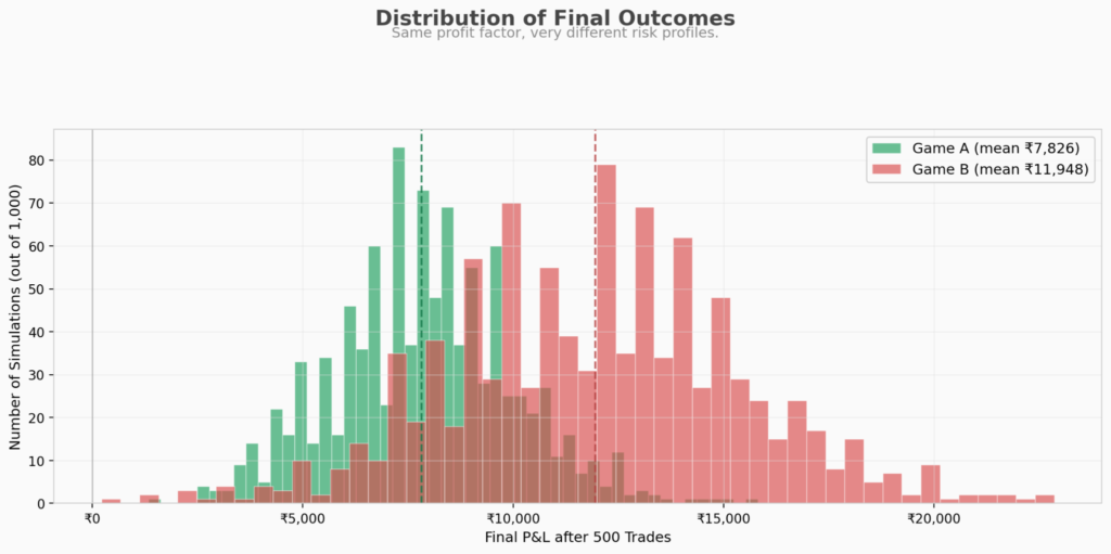
Same profit factor, very different risk profiles
The histogram below shows where you’d end up after 500 trades across all 1,000 simulations. Game A clusters tightly around its mean of ₹7,826. Game B’s mean is higher at ₹11,948, but the spread is enormous. Some runs end near ₹4,000, others blow past ₹20,000.For anyone running a strategy with their own capital, this is not academic. If you’re the kind of person who checks your terminal every hour, Game B will test your conviction in ways Game A never will. The question is not which game is “better”. It’s which game you can actually stick with.
How bad can it feel?
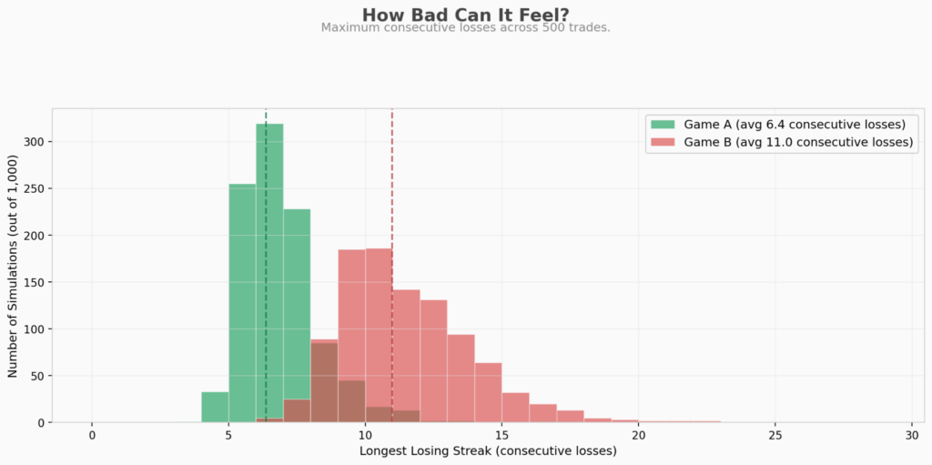
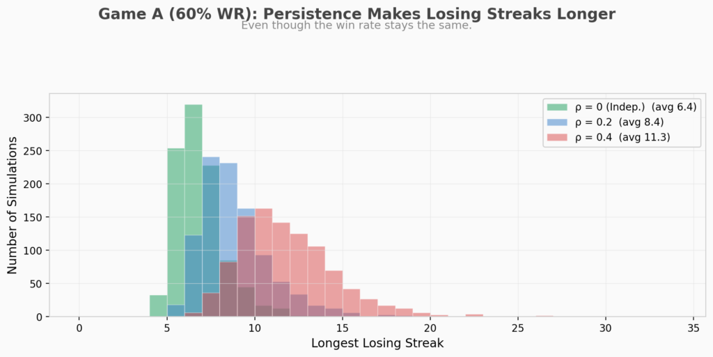
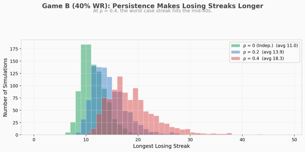
Here’s the part that separates paper traders from real ones. The chart below shows the longest losing streak each simulation experienced across 500 trades.
Game A averages about 6.4 consecutive losses. Uncomfortable, but manageable. Game B averages 11, and regularly hits 15 to 20. If you’re risking 1% of capital per trade, a 20 trade losing streak means watching your account draw down roughly 20% before the strategy even gets a chance to prove itself.
Most traders quit somewhere around loss number 8. Not because the strategy stopped working, but because the emotional pain became unbearable. This is the hidden cost of high payoff strategies. They demand a tolerance for losing that most people simply do not have, unless they’ve trained for it.
But what if trades aren’t independent?
Everything above assumes each trade is an independent coin flip. Win or lose, the next trade starts fresh with the same probability. That’s the textbook assumption. And it’s almost never true in real markets.
Think about what happens during a strong bull run. If your strategy buys trending stocks, several of your positions are likely riding the same tailwind. When one wins, the others tend to win too. And when the regime breaks, the losses come in clusters. Your wins follow wins and your losses follow losses. This is what statisticians call autocorrelation in trade outcomes.
We can model this by introducing a persistence parameter, ρ (rho), that adjusts the win probability based on the previous trade’s outcome.
After a win, the probability of winning again shifts upward.
P(win | last win) = base win rate + ρ × (1 − base win rate)
After a loss, it shifts downward.
P(win | last loss) = base win rate × (1 − ρ)
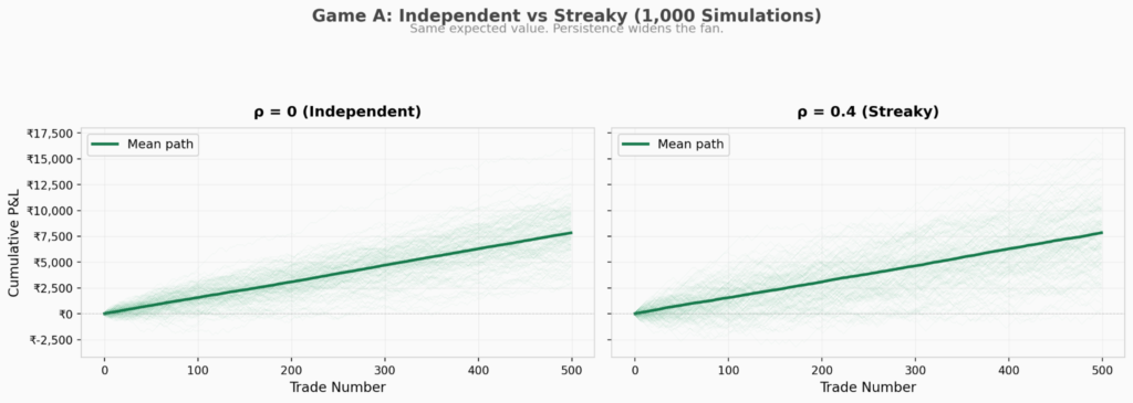
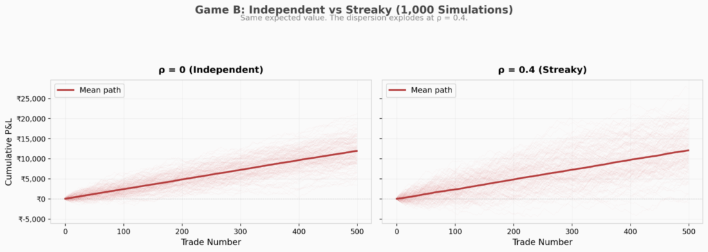
When ρ is zero, the formula collapses back to the independent coin flip. Each trade has the same probability regardless of what came before. When ρ is positive, wins tend to follow wins and losses tend to follow losses, creating the kind of streakiness you’d see in a regime dependent strategy. The important part is that the long run win rate stays exactly the same regardless of ρ. The expected value doesn’t change. Only the path does.
Think of it this way. ρ is a dial that controls how streaky the outcomes are without touching the overall odds. Turning it up doesn’t make the game more or less profitable. It makes it more emotionally volatile.
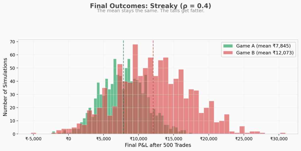
We re-ran the same Monte Carlo simulation with three values of ρ. Zero (our original independent model), 0.2 (mild persistence, roughly what you’d see in a real systematic strategy), and 0.4 (strong persistence, deliberately exaggerated to stress test).
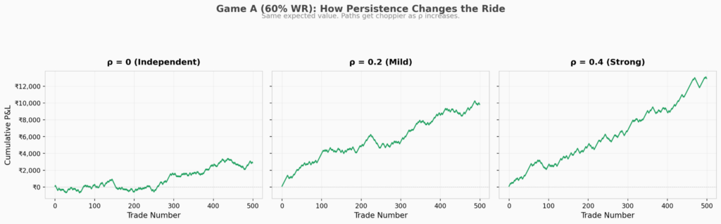
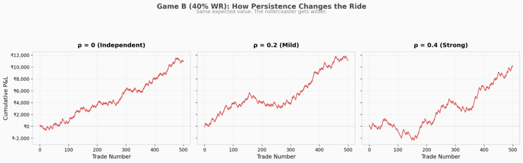
The mean final P&L barely moves. Game A ends around ₹7,800 to ₹8,100 at every level of ρ. Game B hovers around ₹12,000. The expected value is genuinely rho-independent, exactly as the maths predicts.But everything about the experience shifts.
Persistence makes losing streaks worse
The most visceral consequence of autocorrelation shows up in the losing streaks. At ρ = 0, Game B’s average max losing streak is 11 trades. At ρ = 0.2, it jumps to 14. At ρ = 0.4, it stretches to 18, with the worst case in our simulation hitting 43 consecutive losses.
Forty three losses in a row. On a strategy that is provably profitable over the long run.
Even Game A, the “comfortable” game, sees its average max streak nearly double from 6 to 11 as ρ moves from 0 to 0.4. The win rate hasn’t changed. The expected value hasn’t changed. But the psychological torture has.
At ρ = 0.4, profitability across simulations drops slightly. Game A goes from 100% to 99.2%. Game B goes to 99.0%. Still high, but some simulations now actually lose money. The worst outcome for Game A flips from +₹1,338 to -₹2,329. For Game B it goes from -₹90 to -₹5,360. Same edge, but persistence introduces real ruin risk over finite samples.
What we found when we measured our own strategy
We took the win/loss sequence from one of our momentum strategies and computed the lag 1 autocorrelation. Essentially, we asked the question: does knowing whether the last trade won or lost tell us anything about the next one?
The answer was ρ = 0.05. Almost zero.
At first glance, this seems counterintuitive. Momentum strategies exploit persistent trends. Shouldn’t the outcomes be correlated?
The distinction is subtle but important. There is a difference between autocorrelation in prices and autocorrelation in trade outcomes. Momentum exploits the former. A stock that has been trending up tends to keep trending up. That’s the signal, and it’s well documented. But our strategy doesn’t repeatedly trade the same stock. On each rebalance, we rank the entire universe, go long the top decile, hold for the defined period, and then reshuffle. Trade 47 might be a win on Tata Motors and trade 48 might be a loss on Infosys. Those are fundamentally different bets on different companies with different drivers.
Our diversification across names is exactly what kills the autocorrelation. And ironically, that’s a feature, not a bug. A low ρ means our individual trade outcomes are nearly independent. Which means our equity curve converges to the expected value faster and with less dispersion. Remember the Monte Carlo fan charts above. The ρ = 0 fan was tighter than the ρ = 0.4 fan. That tight convergence is what a diversified momentum strategy looks like in practice.
If we were running a concentrated portfolio, say top 5 stocks only, or sector momentum where all positions share common risk factors, we’d see a much higher ρ. The trades would cluster because the underlying drivers are the same. That’s not inherently worse, but it demands a different kind of discipline and a higher tolerance for drawdowns.
Why it matters which game you play
Most people evaluate strategies by win rate alone. That’s like judging a batsman only by how often he scores without looking at his average or strike rate. The win rate tells you nothing without the payoff ratio or the expected value sitting next to it.
A positive expected value means the strategy makes money over a large enough sample. But “large enough” is doing the heavy lifting. Play only 20 rounds of Game B during a bad stretch and you’re deep in drawdown. The law of large numbers guarantees convergence, but only if you stay in the game. And if your trade outcomes are autocorrelated, “staying in the game” means surviving losing streaks that are far longer than the independent model would have you expect.
This is where it gets personal. If you’re a salaried professional running a systematic strategy on the side, you need to ask yourself. Can I hold through 15 consecutive losers without pulling the plug? If the honest answer is no, that doesn’t make you a bad trader. It means you should be running a Game A style system, one that wins more often, even if each win is smaller.
Conversely, if you’ve built the infrastructure to handle deep drawdowns (fixed position sizing, pre-committed capital, automated execution) then Game B’s higher expected value is yours for the taking.
This is precisely why systematic investing exists. A system doesn’t second guess itself after a losing streak. It plays all 500 rounds and lets the expected value converge.Win rate alone is an incomplete metric. A strategy’s real character lives in the interaction between win rate, payoff ratio, and expected value. Layer in the autocorrelation structure of your trade outcomes and you start to understand not just whether a strategy makes money, but what it feels like to run it, and whether you can actually sustain it long enough for the maths to play out. Get that interaction right, match it to a risk profile you can sustain, and the returns follow.