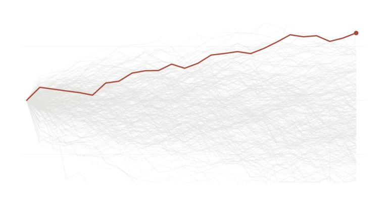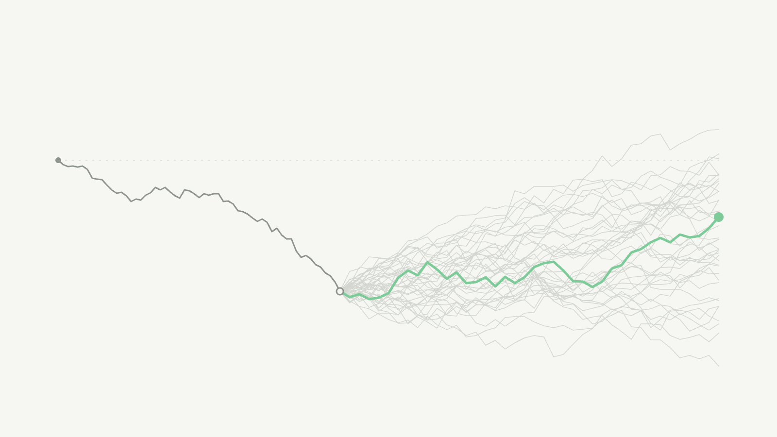

A few weeks ago, in The Nifty doesn’t owe you a rebound, we asked a simple question. The Nifty had just been through a weak five years. Did that mean a strong five years was on the way? Using Nifty data from 1999 onwards, the answer was no. The catch was that India’s market history is short, so the test had only a handful of truly separate five-year periods to learn from. This piece repeats the exercise on a much longer record, the S&P 500 from 1980 to today, to see whether the answer holds up.
Is the market ever “due”?
You have probably heard someone say the market is “due”. The idea goes like this. Stocks have done badly for a few years, so a good stretch must be around the corner, as if the market keeps a record of what it owes you and eventually pays it back.
It is an appealing idea because it feels fair. Markets, though, are not built on fairness. So we tested the idea the way a statistician would, and we will walk through each step so you can see exactly how we reached the answer.
Here is where we ended up. Over 46 years of US data, how the market did in the past five years told us nothing dependable about the next five. Some slumps were followed by the best run in the sample. Others were followed by another slump. Nothing in the slump itself told you which of the two was coming. The same was true when we looked at periods anywhere from one year to ten.
How we set up the test
We started with the daily closing level of the S&P 500 from January 1980 to September 2026. Then we picked a date at the start of every month, from January 1985 to October 2021, and asked two questions about it. How much did the index return per year over the five years before this date? And how much did it return per year over the five years after? Or in other words, the CAGR over the trailing and forward 5 years. Doing this for every month gives us 442 pairs of numbers, one “before” and one “after” for each date.
If bad periods really set up good ones, a low “before” number should usually come with a high “after” number. Put all 442 pairs on a chart and the dots would drift downward from left to right. That is the pattern we were looking for.
What the raw data shows
Start with a simple count. When the past five years were below average, the next five years came in above average 63% of the time. When the past five years were above average, the next five came in above average 60% of the time. A gap of three percentage points is small enough that luck can easily explain it.
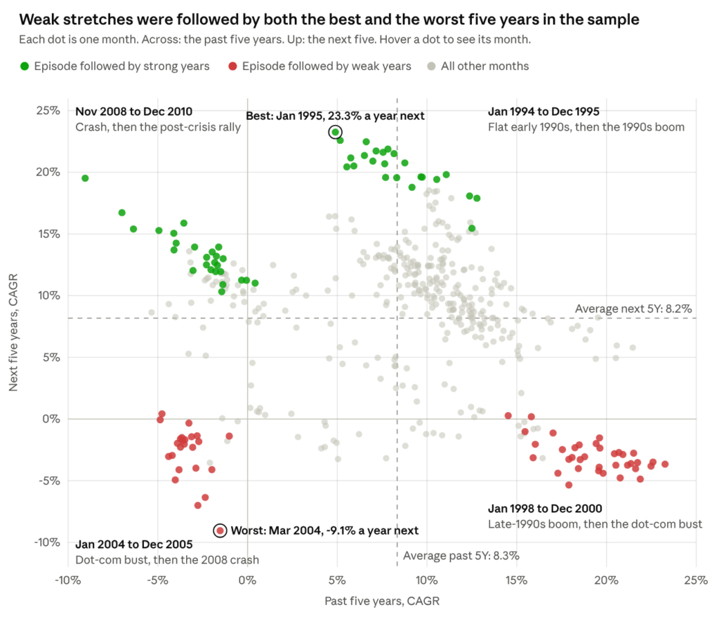
Each dot on this chart is one month. How far right it sits tells you the return over the five years before that month. How high it sits tells you the return over the five years after. The two dashed lines are the averages, about 8.3% a year for the past five years and 8.2% for the next five. Out of 442 months, 218 flipped to the other side of the average and 224 stayed on the same side, which is almost an even split.
The coloured groups are four stretches of history worth looking at closely. Start on the left side of the chart, where the past five years were poor. The green dots there are months from November 2008 to December 2010. Anyone investing then had just lived through the financial crisis, and the next five years brought a strong recovery. The red dots below them are months from 2004 and 2005. Those investors had just lived through the dot-com crash, and their next five years ran straight into the 2008 crisis. Both groups started from a slump. One got a rebound and the other got a second slump.
The other two groups tell the story of the 1990s. Months in 1994 and 1995 came after a few flat years and were followed by the great late-1990s boom, which includes the single best five years in the sample. The red dots on the far right are the end of that boom, from 1998 to 2000, and the five years after them were the dot-com bust.
If you take the worst quarter of all the trailing periods and average what came next, you get 6.6% a year. That is lower than the 8.2% average across all months. So on average a slump was followed by slightly below-average returns, which is the opposite of a catch-up.
Why 442 dots are not 442 pieces of evidence
There is a catch in that chart, and it matters a lot. Take two neighbouring dots, say March and April of the same year. The five years before March and the five years before April share 59 of their 60 months. So the two dots are almost the same measurement taken twice. That is why the dots line up in slow trails rather than scattering on their own. Over 46 years, you can only fit about seven five-year periods that do not overlap at all.
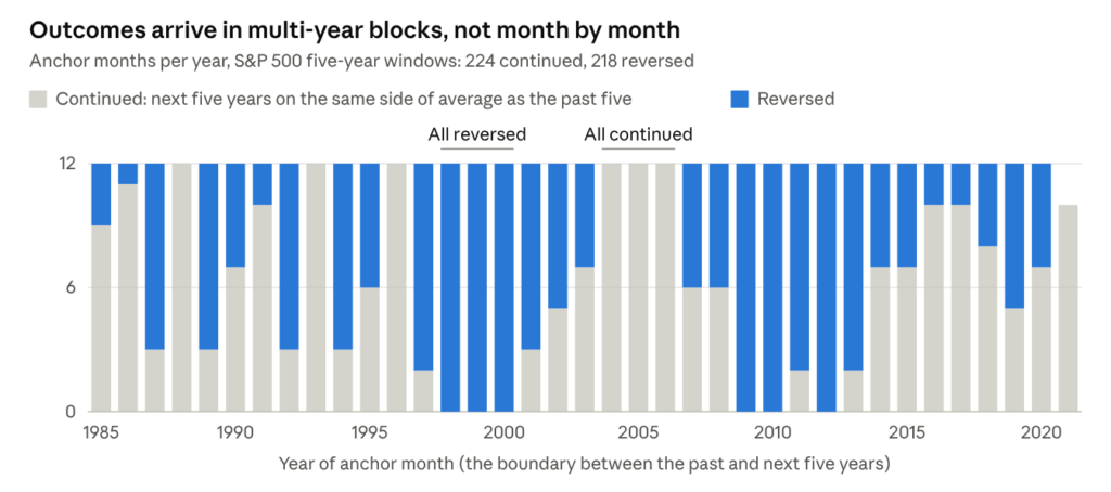
This chart shows the same thing year by year. For three straight years in the late 1990s, every single month flipped to the other side of the average. From 2004 to 2006, every single month stayed on the same side. Each of those blocks is really one event counted 36 times.
Why does this matter? Standard statistical tests assume that every data point brings new information. Feed them 442 heavily overlapping dots and they become far too confident. At the 10 year horizon, for example, a standard test says past returns explain 33% of future returns and puts the odds of that being luck at practically zero, but with such sparse data points at the 10 year horizon, it is difficult to be confident about the r-squared figures of 33% . As the next section shows, a market with no memory at all produces a pattern that strong roughly one time in three.
A fair comparison: markets with no memory
To know whether the real pattern means anything, we need something to compare it with. So we built simulated versions of the S&P 500 in which the past cannot possibly affect the future. We took the 561 actual monthly returns from 1980 to 2026, put them in a hat, and drew them out at random, with replacement, until we had a new 46-year history. Every month in that history is real, crashes like October 1987 included. Only the order is random, so a bad stretch has no way of causing a good one.
Then we ran exactly the same calculation on the simulated history as on the real one with the same dates, the same five-year windows, the same chart. We repeated this 10,000 times. The result is a picture of every pattern that overlap and plain luck can produce on their own.
The first surprise is that the simulated markets also show a downward slope on average, even though nothing in them can bounce back. That slope is created by the overlapping windows and the short sample, and it gets steeper the longer the period you look at. It also sets the bar for the real data. The real S&P 500 pattern only counts as evidence if it is more extreme than what the simulated markets usually produce.
Shorter and longer periods
Five years is an arbitrary choice, so we repeated the whole test for every period length from one year to ten. In the chart below, the blue dot is the real S&P 500 and the grey bar is the range the simulated markets produced. At every length, the blue dot sits comfortably inside the grey bar. The closest call is three years. The smallest p-value is 0.32, which means about a third of the simulated markets produced a stronger pattern than the real one.
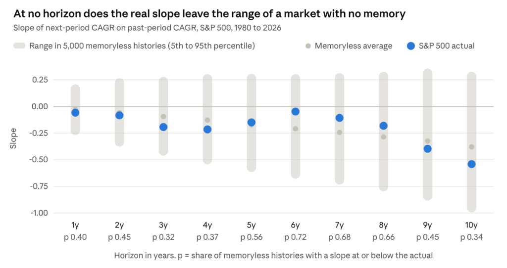
Notice how the small grey dots, the average of the simulated markets, slide lower as the period gets longer. That is the overlap effect from earlier, and it accounts for most of the steep real slopes at nine and ten years.
Looking at slumps and booms separately
There is one more way a real pattern could hide. Suppose slumps were followed by rebounds while booms were followed by even more gains. Those two effects point in opposite directions and could cancel each other out on a single chart. To check, we split the months into two groups at the average past return of 8.3% a year and drew a separate regression line through each group.
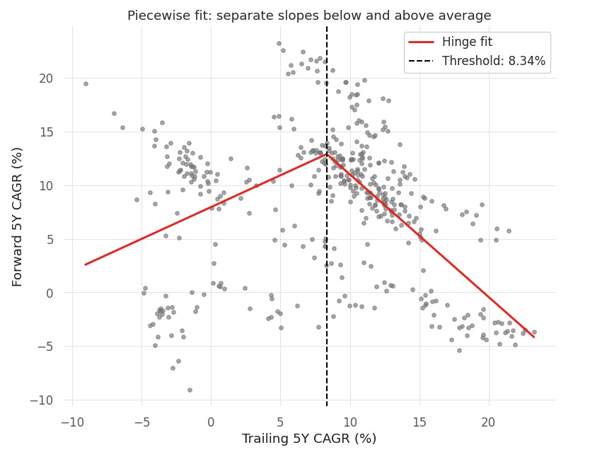
Looking at the left-hand line first, it covers the months that came after a weaker-than-average five years. If slumps were repaid, this line would rise as you move left, because a deeper slump would bring a bigger rebound. It does the opposite. A five-year stretch 10 points below average was followed, on the line, by about 7% a year. The worst stretch in the sample, about minus 9% a year, was followed by about 2.6% a year. The deeper the slump, the weaker the years that followed, and this held in every version of the test we ran.
The right-hand line covers the months that came after a stronger-than-average five years, and here the line falls steeply. A stretch of about 18% a year was followed, on the line, by roughly 1.5% a year. Only one or two make-believe markets in a hundred produced a pattern that strong. Almost all of it, though, comes from one period, the late-1990s boom and the dot-com crash that followed. If we remove the 48 months from 1997 to 2000, the pattern shrinks by more than half, and about one in four make-believe markets then produces something at least as strong. What looks like a rule about booms is really the story of one bubble.
Why did the 2000 crash and the 2008 crash lead to such different futures? Our data cannot answer that, but the most likely explanation is price. In 2000, US stocks were more expensive relative to company earnings than they had ever been. The crash that followed brought prices down, but not far enough to make stocks cheap, and the next five years were poor as well. In early 2009, stocks were much cheaper, and a strong recovery followed. This fits what the Nifty piece found when it split returns into earnings growth and changes in valuation. If it holds, what drives future returns is the price you pay, and how the last few years felt tells you very little.
What this means for you
A bad year, or even a bad five years, does not put the market in your debt. If you buy more shares after a slump, do it because you have a long horizon and stocks have rewarded patient investors over long periods. Do not do it because you think a bumper year is owed to you. For planning, the roughly 8% a year this sample delivered on average is a far more honest number than any catch-up you might hope for.
The same reasoning works in the other direction. A strong run was not, by itself, a good reason to sell. After above-average five-year stretches, the next five years still beat the average 60% of the time. Only the most extreme bubble in the sample was followed by a clear bust.
What does help is deciding how much of your money belongs in equities based on your time horizon, when you will need the cash and how large a fall you can sit through, and then rebalancing on a fixed schedule. If you want a signal from the market, starting valuations have a much longer track record in academic research than recent returns. This piece is research, not investment advice.
Technical appendix
All inference here comes from a simulated null, because overlapping windows make textbook standard errors invalid. The design follows the long-horizon literature (Fama and French 1988, Poterba and Summers 1988) and its small-sample critiques (Richardson and Stock 1989, Valkanov 2003).
Data and construction. S&P 500 price index, nominal, from daily closes, January 1980 to September 2026. At each monthly anchor, the trailing leg is the CAGR over the preceding h years and the forward leg the CAGR over the following h years, for h from 1 to 10. At h = 5 this gives 442 anchors, January 1985 to October 2021.
Specifications. The linear test and the piecewise (hinge) test, where x is the trailing CAGR and c its sample mean (8.34%):
fwd_t = alpha + (beta)*(x_t) + error_t
fwd_t = alpha + (beta_low)*(min(x_t – c, 0)) + (beta_high)*(max(x_t – c, 0)) + error_t
Residuals are almost perfectly autocorrelated (Durbin-Watson 0.08 in the hinge fit), which is the overlap at work. At h = 5 the linear fit gives a slope of minus 0.149 with R-squared 0.023. Its textbook p-value is 0.001, while the simulated p-value is 0.56.
Null distribution. An IID bootstrap of the 561 monthly log returns, drawn with replacement. Each simulated history is rebuilt into a price path and pushed through the identical pipeline, with the hinge threshold recomputed inside each history. We ran 5,000 histories per horizon and 3,000 per robustness check. A p-value is the share of simulated slopes at or below the real one, unless marked otherwise.
Robustness of the piecewise test (h = 5).
| Variant | Above-average slope | p (left tail) | Below-average slope | p (right tail) | Difference p (two-sided) |
|---|---|---|---|---|---|
| IID bootstrap, threshold at mean | -1.14 | 0.014 | 0.59 | 0.041 | 0.020 |
| Block bootstrap, 12-month blocks | -1.14 | 0.020 | 0.59 | 0.044 | 0.021 |
| Block bootstrap, 24-month blocks | -1.14 | 0.023 | 0.59 | 0.026 | 0.013 |
| Threshold at median (9.65%) | -1.29 | 0.010 | 0.47 | 0.073 | 0.018 |
| Threshold at mean minus 2 (6.34%) | -0.97 | 0.020 | 0.83 | 0.024 | 0.015 |
| Threshold at mean plus 2 (10.34%) | -1.39 | 0.014 | 0.41 | 0.071 | 0.021 |
| Anchors 1997 to 2000 removed | -0.49 | 0.25 | 0.58 | 0.057 | 0.17 |
| Anchors 1997 to 2001 removed | -0.42 | 0.32 | 0.61 | 0.050 | 0.20 |
Multiple testing. About 14 tests were run across this study. The above-average slope, at p of 0.01 to 0.02, does not clear a Bonferroni threshold of 0.0036. The below-average slope was specified in advance as a test for reversal (left tail), so the continuation it shows is a hypothesis for other markets, not a finding.
Limitations.
- One market, and the winning one. The S&P 500 recovered from every drawdown in this window, which biases the sample toward rebounds. That no rebound effect appears anyway makes the result stronger, not weaker.
- Low power. About seven independent five-year episodes cannot rule out a modest effect. A power analysis on a simulated mean-reverting market would show the smallest effect this sample could detect.
- No valuation control.